If you look in a modern treatment of optimal transportation, you will likely find the problem defined as something like $$ W_c(\mu,\nu) = \inf_{\pi \in \Pi(\mu,\nu)} \int_{X \times Y} c(x,y) d\pi $$ This is the modern definition of the problem, where we model the objective as finding the minimum cost coupling between $\mu$ and $\nu$. But this is not the original formulation of the problem. Before Kantorovich blessed us all with modern probability theory, Gaspard Monge first proposed that we intead consider $$ \inf_{T : T_{\# \mu} = \nu } \int_{X} |T(x) - x| d\mu $$
$$T_{\# \mu}(A) = \mu(T^{-1}(A)) = \nu(A) : \underbrace{\forall A \subset X}_{measurable} $$
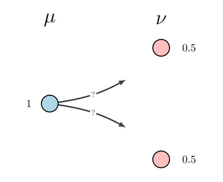
In the case of the Euclidean squared cost, i.e $c(x,y) = |x-y|^2$ and $\mu$ being absolutely continuous with respect to the Lebesgue measure, the celeberated Brenier theorem tells us that these two formulations yield the same results. But most of the time, this is not the case. Indeed, the ubiquitous counterexample to the equivalence of these formulations is to consider the discrete problem where $X =\{x\}$, $\mu = \delta_{x}$, $Y = \{y_1,y_2\}$ $\nu = \frac{1}{2}\delta_{y_1} + \frac{1}{2} \delta_{y_2}$

In this example, since a function cannot be multi-valued, clearly no transport map can exist.
While Kantorovich’s formulation is undeniably the “correct” one, in that it always has a solution (under very mild assumptions on $\mu$ and $\nu$), in some situations it might be interesting to consider how close we could get by still requiring a deterministic map (i.e ignoring plans). Of course, we would need a way of “softening” the constraint that $T_{\# \mu} = \nu$, since it might not always be possible to satisfy it. Instead, we could consider
$$ \inf_{T \in L^2(X)} \left ( \int_{X} |T(x) - x|^2 d\mu + \gamma\Gamma (T_{\# \mu}, \nu) \right)$$ where $\Gamma$ is some regularization term that penalizes $T_{\# \mu}$ for differing from $\nu$.
What could we use for $\Gamma$? Some options might be
While the KL divergence might seem attractive due to its closed form expression, the obvious issue is that when $T_{\#\mu}$ is not absolutely continuous with respect to $\nu$, the divergence is not defined (the Radon derivative in the logarithm ceases to make sense). This seems likely to be a problem if we wish to solve this problem algorithmically (which is why I’m writing this), since imposing the constraint that our maps must hit the support of $\nu$ *exactly* would be difficult, if not downright impossible in practice.
So, why not loosen up a bit? Another option is the Total Variation Norm, which, being a norm and therefore a proper metric, does not suffer from the affliction of exploding values as KL does if $T$ is to miss the support of $\nu$. However, as is also well know, it $TV$ is as well too strong to give useful information about the proximity of $T_{\# \mu}$ to $\nu$ in the sense we want to assess, the canonical example being for any two dirac masses $\delta_{x}, \delta_{y}$ on the real line, we have $$ TV(\delta_{x}, \delta_{y}) = \sup_{A \text{ measurable }} |\delta_{x}(A) - \delta_{y}(A)| = 1 : \forall x \neq y$$ which goes back to one (of many) of the main reasons that optimal transportation is intriguing. Formally, of course, this is because the Wasserstein (or Kantorovich if you’re a pedant) metric lifts the ground distance to the space of distributions, and so avoids giving us constant values invariant of the geometry of the supports. In our case, this is desirable because we want to know how *much* we are missing the target distribution by requiring our transport plans to be maps.
While it might seem odd at first, given that we wanted to consider how well we could do with maps and not plans, using $W_c$ as our $\Gamma$ regularizer has a few key advantages. First, as mentioned above it captures desired metric of similarity via metrizing weak convergence. Second, while computing it can be unwieldy due to the classic algorithm scaling $O(n^3)$ in the number of points in the support of $\mu$ (we will have to restrict our attention to discrete distributions to have any hope of computing anything), new approaches using entropic regularization have improved that cost to $O(n^2/\varepsilon)$ for a $ O(\varepsilon)$ close approximation.
Indeed, this is the approach presented in Perrot et al, 2016, which in part inspired this post. However, instead of learning the dual potentials as they suggest, we could implement the Sinkhorn algorithm as a step in our loss function (akin to what Genevay et al, 2018 propose for generative models), then use automatic differentiation to compute our gradients for our optimizers.
I don’t generally prove much in these posts, but I feel there is one lemma worth at least sketching. If we fix our map estimation problem as $$ \inf_{T \in L^2(X)} \left ( \int_{X} |T(x) - x|^2 d\mu + \gamma W_2 (T_{\# \mu}, \nu) \right) $$
Assume $\nu,\mu$ have second order moments. Then if there does exist a transporation map $T^*$ such that $T^*_{\#\mu} = \nu$ and $T^*$ minimizes the first term, then that $T^*$ also minimizes the entire expression. This follows somewhat trivially because then, $$ W_2(\mu,\nu) = \int_X |T^*(x) - x|^2 d\nu \leq \int_X |T^*(x) - x|^2 d\nu + \underbrace{\gamma W_2(T^*_{\#\mu}, \nu)}_{=0} $$ where $W_2(T^*_{\#\mu}, \nu) = 0$ follows because under these conditions, $W_2$ is a metric on $\mathcal{P}_2(X)$. But this also means $W_2$ satisfies the triangle inequality, thus for any $T$ (regardless of what the measure $T^*_{\#\mu}$ happens to be), $$ W_2(\mu, \nu) \leq W_2(\mu,T_{\#\mu}) + W_2(T_{\#\mu},\nu) \leq \int_{X} |T(x) - x|^2 d\nu + \gamma W_2(T_{\#\mu},\nu) $$ under the mild assumption $\gamma > 1$. I would expect to also be able to show convexity of the objective by using similarity machinery.
Consider each term in this equation separately: $$ \inf_{T \in L^2(X)} \left ( \underbrace{ \int_{X} |T(x) - x|^2 d\mu}_{(1)} + \underbrace{\gamma W_c (T_{\# \mu}, \nu)}_{(2)} \right) $$
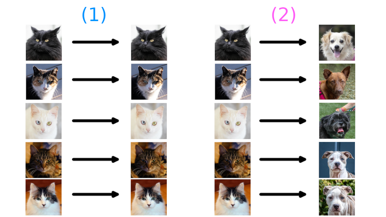
To give an intuitive explanation of what this is saying: Imagine we have two distributions, one made up of images of cats and one made up of pictures of dogs. The maps $T$ then map from images to images.

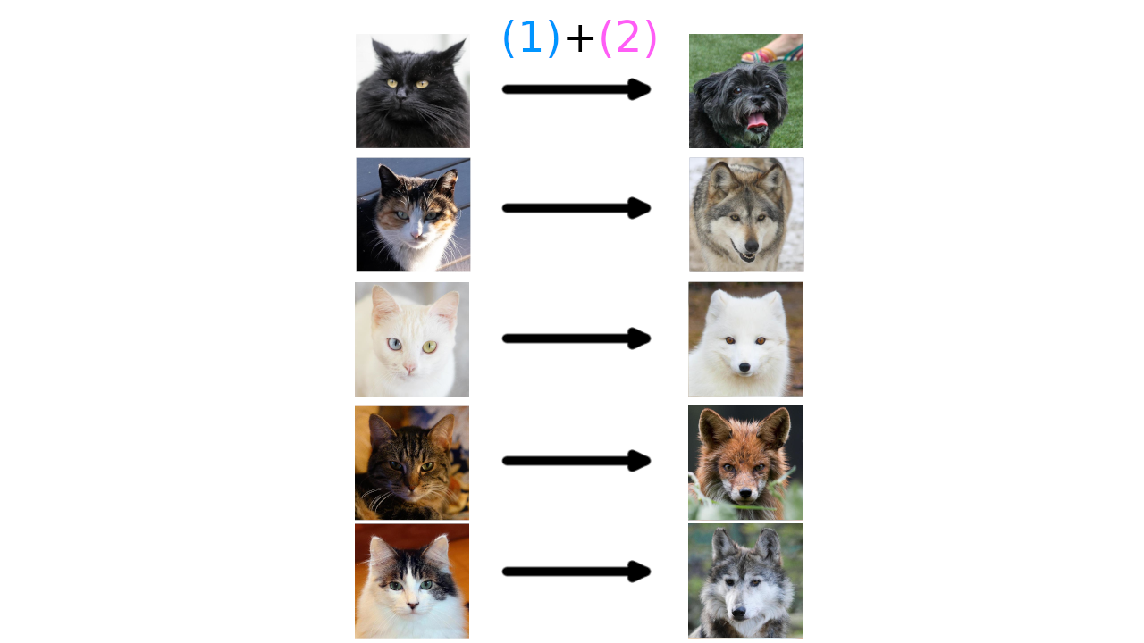
If I gave you images of cats and asked you to give me a set of pictures (images) that were the closest to those pictures, you would probably just give me back the same pictures. This is the result of minimizing (1). Similarly, if I gave you pictures of cats and asked you to make them into pictures of dogs, you could just randomly choose a dog for each cat. This is the result of minimizing (2). Either objective alone isn’t particularly interesting. But by pitting these objectives against each other, the minimizer would have to (1) not produce dogs too different than the cats and (2) produce dogs that look like dogs.
 Here you can see that only one of the target pictures is actually a dog, the rest are wolves. In general this is what we should expect when trying to learn a transportation map on a discrete space; hitting the target exactly will likely be impossible.
Of course, if we are interested in this problem from a computational perspective, the question you should have in mind is: why? Well, one reason that seems hot at the moment (or was within the last few years) is that computing maps from a source to a target destination is the underlying problem that Generative Adversarial Networks seek to address. Indeed, as commonly formulated, the idea of a GAN is to find the best mapping from a noise distribution onto one given by samples from a dataset, with the critic being trained to determine the best. GANs are beyond the scope of this article (and perhaps most mathematical analysis), however, we don’t need such complicated scenarios to imagine where learning good distributional mappings may be of interest.
One good example is dataset augmentation. If I have a large dataset $A$, which captures a range of examples that are interesting, and a smaller set $B$, which we wish to enlargen, we could learn a map via this process that takes instances of $A$ close to instances of $B$. However, by setting the parameters correctly ($\approx$ lower $\gamma$), the map (at least ideally) will generalize beyond just returning instances of $B$.
Alternatively, we could use this as a type of fuzzy classification, with higher penalization $\gamma$ to enforce the output being close to the target distribution (say clusters of examples from the classes). In this case, we would hope that the penalization in the (1) term would help the model generalize better, because, loosely speaking, it enforces a type of regularity on the map $T$.
All this is of course very vague, but that’s kind of the point. There are a lot of potential applications that fit within this framework, given the proper formalism. The last example perhaps illustrates how this formulation can be thought of as a fuzzy matching problem; a relaxation of optimal transport that could be used to fit many problems in data science and beyond.
Stepping back into the land of theory, the other benefit here is that by formulating problems in this framework, we have access to an enormous literature of theorertical optimal transportation that can be adapted to these problems. This could help give guarantees and proofs of techniques that would be hard or impossible to handle in their original presentations.
We will detail some toy implementations here in the future.